3.1. Fly Base and Gbrowse
As we mentioned previously, transposable elements are DNA sequences that jump from one part of the genome to another; and constitute a kind of mutation. When a TE is discovered, we assign it a name.
In Drosophila melanogaster, all genomic information, including the TE sequences, is gathered into a huge database. This database is called Fly Base – which is a surprise, isn’t it? To make it simpler, each TE has an identifier (ID) inside the database.
Each TE starts by FBti (Fly Base Transposable Insertion) followed by a unique number: for example FBti0019099
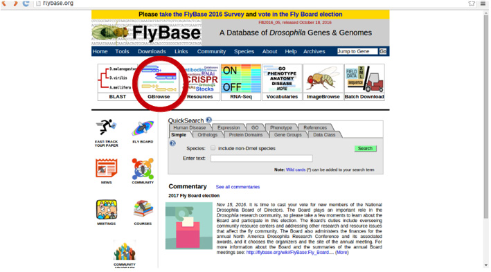
With GBrowse, you can visualize the genetic information of a specific place in the genome. You can also easily browse around and move through different genomes and their characteristics. Do you want to try it? Why don’t we look for the previously mentioned TE using the Drosophila melanogaster GBrowse? Let’s see where TE FBti0019099 is located, and which genes are nearby.
For this purpose, we have to visit Flybase.org. We need to click on the second option in the upper panel: GBrowse.
Once there, in ‘Landmark or Region’ we can write the name of our TE: FBti0019099:
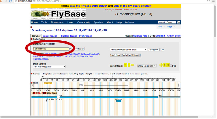
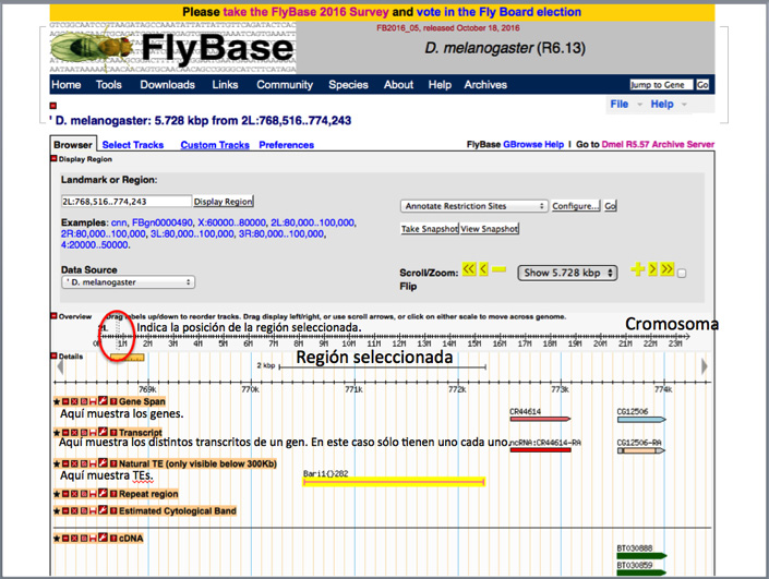
Using the zoom option, you can zoom in or out of a specific region to check what surrounds the ~6,000 bp region shown by the GBrowse by default.
Genetic Measures
- A base pair (bp) is a pair of nucleotides and it points to a unique region in the genome.
- A kilobase (kb) is a 1,000 bp.
- A Megabase (Mb) is a 1,001 kb or 1,000,000 bp.
You are free to play around and explore within the browser a bit. If you you´re not sure how to return to where you began, you can always write the TE ID (FBtiXXXXXXX) into the search box again, and you will be returned to the starting ~ 6,000 bp.
Mediante la pestaña del zoom podéis ampliar o reducir la región para ver que hay más allá de las ~ 6000 pb que el GBrowse muestra por defecto.
3.2. What Does the Data File Include?
Attached is a data file, which contains a list of specific TE groups found in the Drosophila melanogaster genome. As we said before, most mutations are deleterious, and as a result of this, they will be present at low frequencies in the genome. Very few individuals (sometimes one or two) will carry those mutations. We suspect that there are around 20,000 TEs in each Drosophila population. Current scientific tools allow us to detect and estimate the frequency of 1,632 of these TEs, due to these sequences being highly repetitive and easier to distinguish between them. However, these 1,632 TEs are not the only TEs present in the genome, but only the ones we can currently work with.
Previous generations of scientists could only analyze very specific TE cases. Now, we can analyze all 1,632 TEs together. Maybe, by the time you become a scientist, you could analyze all the ~ 20,000 TEs yourself!!
The data file contains information for all 1,632 TEs, and it is divided into the following columns:
- TE ID (TE_ID).
- Name (Tename).
- Chromosome (chr) where the TE has inserted the genome.
- Starting position on the chromosome (start).
- Ending position on the chromosome (end).
- Recombination levels in the specific region where the TE is in the genome
- Distance (in bp) to the closest gene. When distance is 0, the TE is inside or partly overlapping the closest gene. You can check for examples of this by searching the following in GBrowse: FBti0019985 or FBti0019017.
- The closest gene ID.
- This gene name.
- – 14. TE frequency in 5 different populations. One Zambian (African) – the population where flies are thought to originate from (column 10), and 4 European populations: Portugal (Recarei) in column 11, Spain (Gimenells) in column 12, Germany (Munich) in column 13 and Finland (Akaa) in column 14.
Save it locally to your computer and let’s work with it!!
3.3. How do we import our data file into R?
First things first, we have to import our data file in R.
To do this, you can use the following function that you can also find in the R code file:
Data_file <- read.delim(file=”~data_file.txt”, head=TRUE)
In the code file (which you already downloaded in module 2.4) you can find real examples where you can use these kinds of functions. You will have to copy the function into your own code file that you opened in your text editor. Then you have to change the path – the location in your computer – to where you downloaded or saved the data file. After this, you can just copy and paste it into the R console (left box highlighted in red).
How to make conditions in R:
- Equal to: ==
- Different to: !=
- Greater than: >
- Lower than: <
- For multiple conditions and the same time, you can use & (and) or | (or)
If you can’t import the file with this function, you can use the following method instead:
Use the Import Dataset tab in the upper right box (“environment”). Select option “From Text (base)…”.

Click on Browse and select the data file from your computer.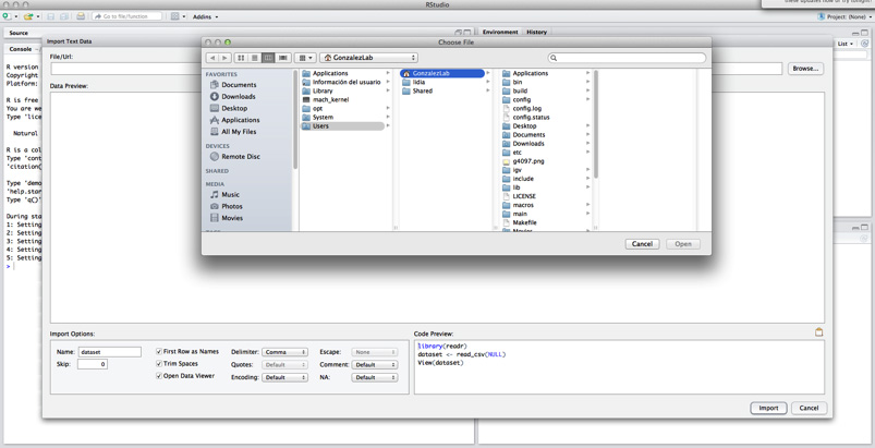
Finally, you have to set your file as tab-delimited, and change option “Quotes” to “none”.
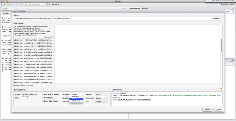

Click Import.
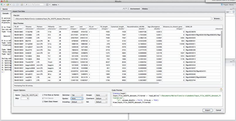
If you have done it properly, you will see your file in the upper left box of the program. Now you can start working in R!!
Here you have a brief description of each screen function and information on each of them.
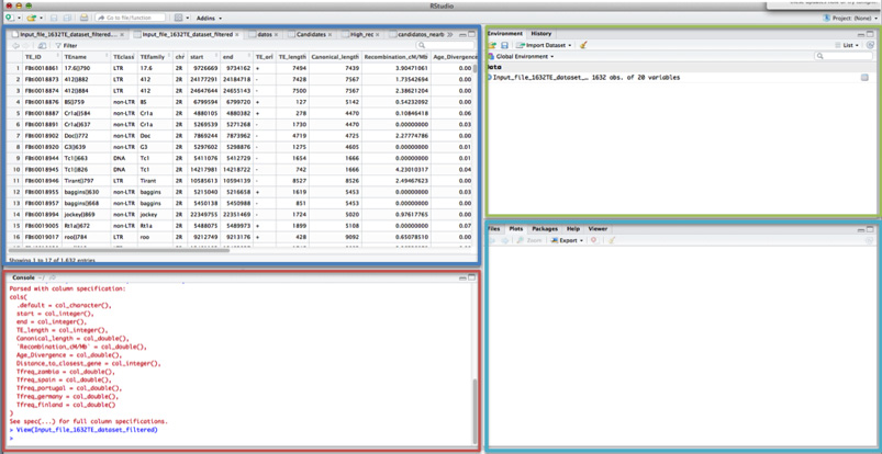
The most important part of the screen is the RED BOX: console or terminal. This is where you have to paste all the commands you want to execute in R.
REMEMBER: the conditions in R are:
- Equal to: ==
- Different to: !=
- Greater than: >
- Lower than: <
- For multiple conditions and the same time, you can use & (and) or | (or)
Although RStudio allows you to save the executed commands from the terminal, we advise you to copy all the working commands into a different file; opened and saved in the text editor. In this way, you can keep on working on the same file on different days or with different computers. You will need to have your own code file formatted like ours, but customized by you. With that, you’ll only have to copy and paste all your commands and you can start working from the same place you left off.
In the BLUE box, you can visualize all the information on the data file. In each of the different tabs, you will have all the new datasets you will either import or create.
In the GREEN box you will have 2 tabs:
- Environment, where you can see all the different datasets you will open or generate in R
- History, where all the commands you have tried, including those that work and those that do not, are saved.
This is why we advise you to save the commands that you are sure are working into a different file. So, at the end, you’ll know which of these commands are really important for your work.
In the PURPLE box, you will find different tabs. If you select the “Plots” tab, you can see all the different plots and figures you´ve created.
3.4. Distribution of Variables of Interest
Now that our data has been properly imported into the program, we can start analyzing the distribution of variables that we have in our data file.
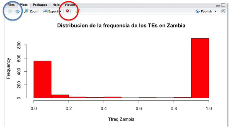
Do you know what the TEs frequency distribution is in each of the 5 sequenced populations? Let’s do a histogram so we can see it easily.
hist(data_file$Tfreq_zambia)
This function can be found in the example code file that you can open in the text editor.
You can change the colors: check out how to use your favorite ones here.
If you want to keep trying and modifying the graph, you can check out this other page.
Now, let’s see how the TEs are distributed in other populations. Each graph shows up in the same box, with arrows in the upper part of the box that allow you to change from one graph to another. By using the “X” button (“Remove the current plot”) you can delete graphs.
3.5. TEST YOURSELF